5 Utility functions
5.1 poolLengthComp function
The poolLengthComp function pools length data when multiple columns exist. It sums length frequency data or concatenates length composition data as a single vector. This function is used within other functions, and is typically not called directly by the user.
5.2 LoptFunc function
The LoptFunc function calculates optimum harvest length. Derived from Beverton (1992), in a year-class subject to a moderate and constant exponential mortality and whose individuals are growing towards an asymptotic size (as in the Von Bertalanffy growth function), the total biomass of the year-class (i.e. the product of numbers and average weight) reaches a maximum value at some intermediate age (\(Topt\)) at a certain weight and length of the individual fish (\(Wopt\) and \(Lopt\), respectively). \(Lopt\) is calculated as:
\[
Lopt = 3 \frac {L_{\infty}}{(3 + M/K)}
\]
This function is necessary for the PoptFunc function (proportion of fish within optimal sizes in the catch).
5.3 LcFunc and modeKernelFunc functions
These functions estimate length at full selectivity from a LengthComp object. This can be done in two methods: 1) using the mode of the length-frequency distribution (LFD); or 2) applying a Kernel smoother to the LFD.
In the first method the cumulative distribution of the LFD is computed, and a loess smoother is applied to predict across equally spaced length intervals (1 unit interval, i.e., 1 cm interval); the length at which the cumulative distribution of the predictions increases the most (highest slope) corresponds to the mode of the LFD (Babcock 2013). Figure 1 shows the cumulative distribution of an example predicted LFD, and the vertical line corresponds to the mode of the distribution.
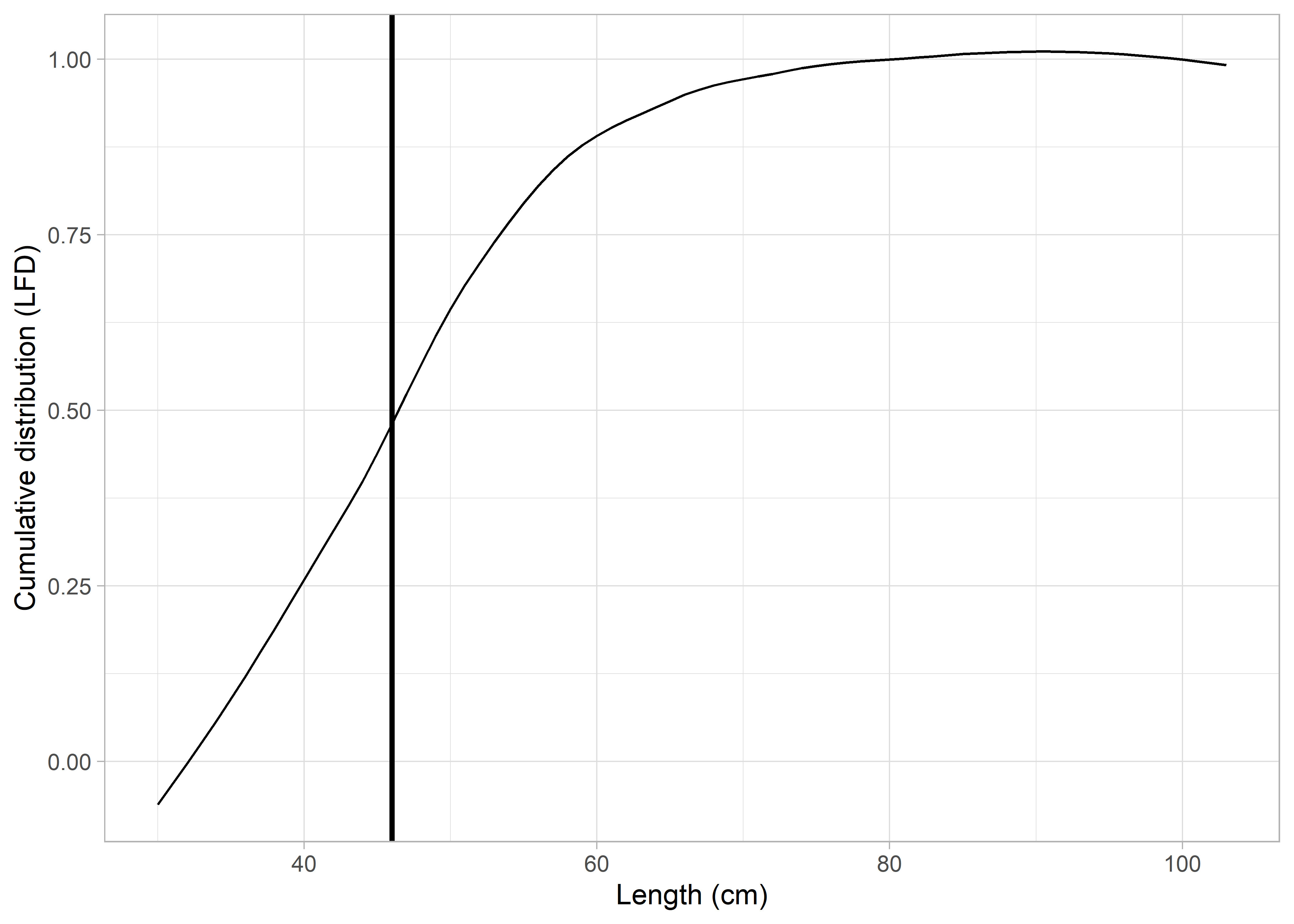
Figure 5.1: Cumulative length-frequency distribution
In the second method a Kernel smoother is applied to the LFD and its maximum value is taken as the length at full selectivity. Figure 2 shows the length at which the Kernel smoother estimates highest density estimates.
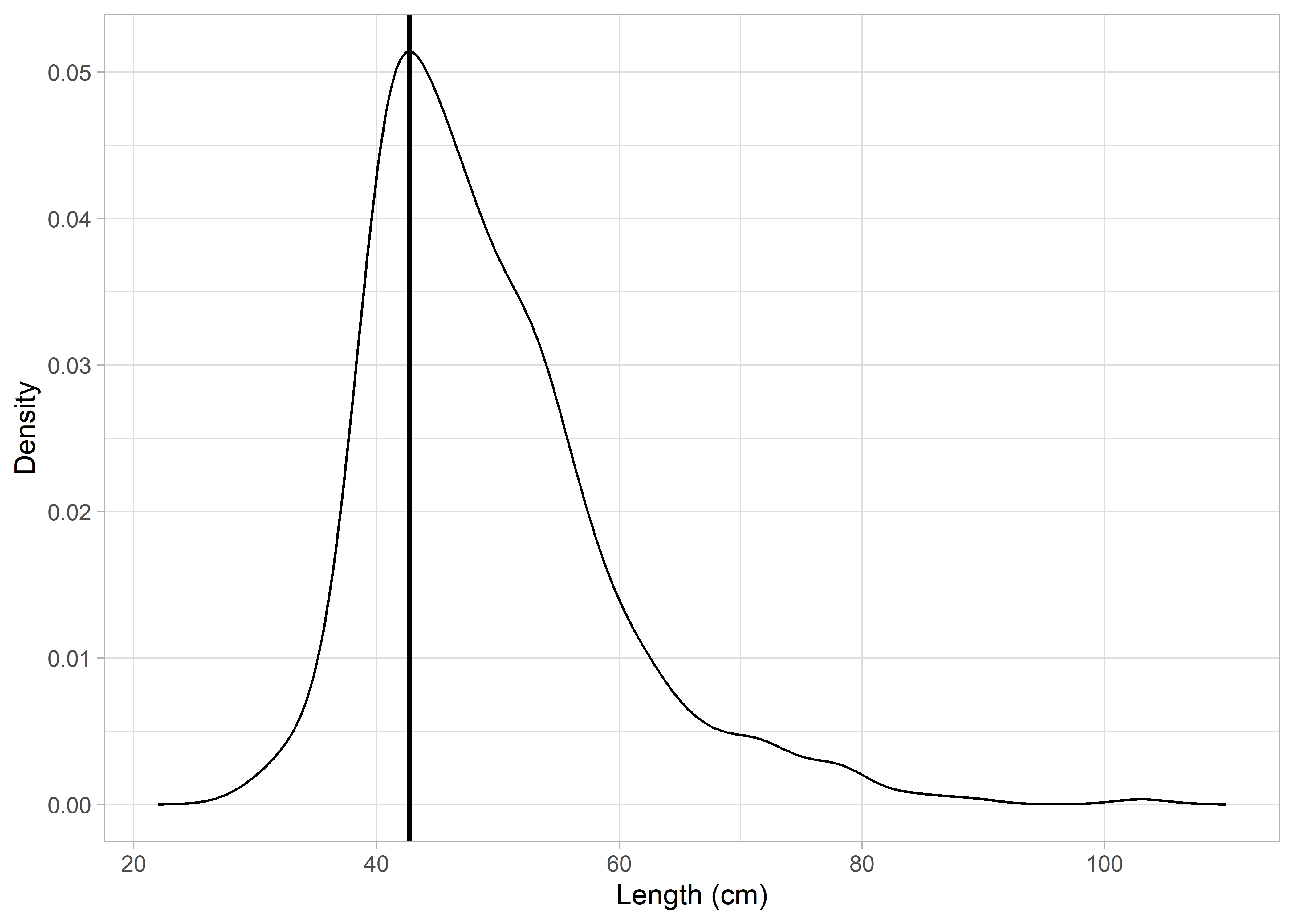
Figure 5.2: Kernel smoother applied to length-frequency distribution
Some results from applying these two functions to example LFDs are presented below. The left-hand plots show an example LFD, and the right-hand side plots show a subset of the example LFD, in order to test the functions with smaller sample sizes and more sparse data.
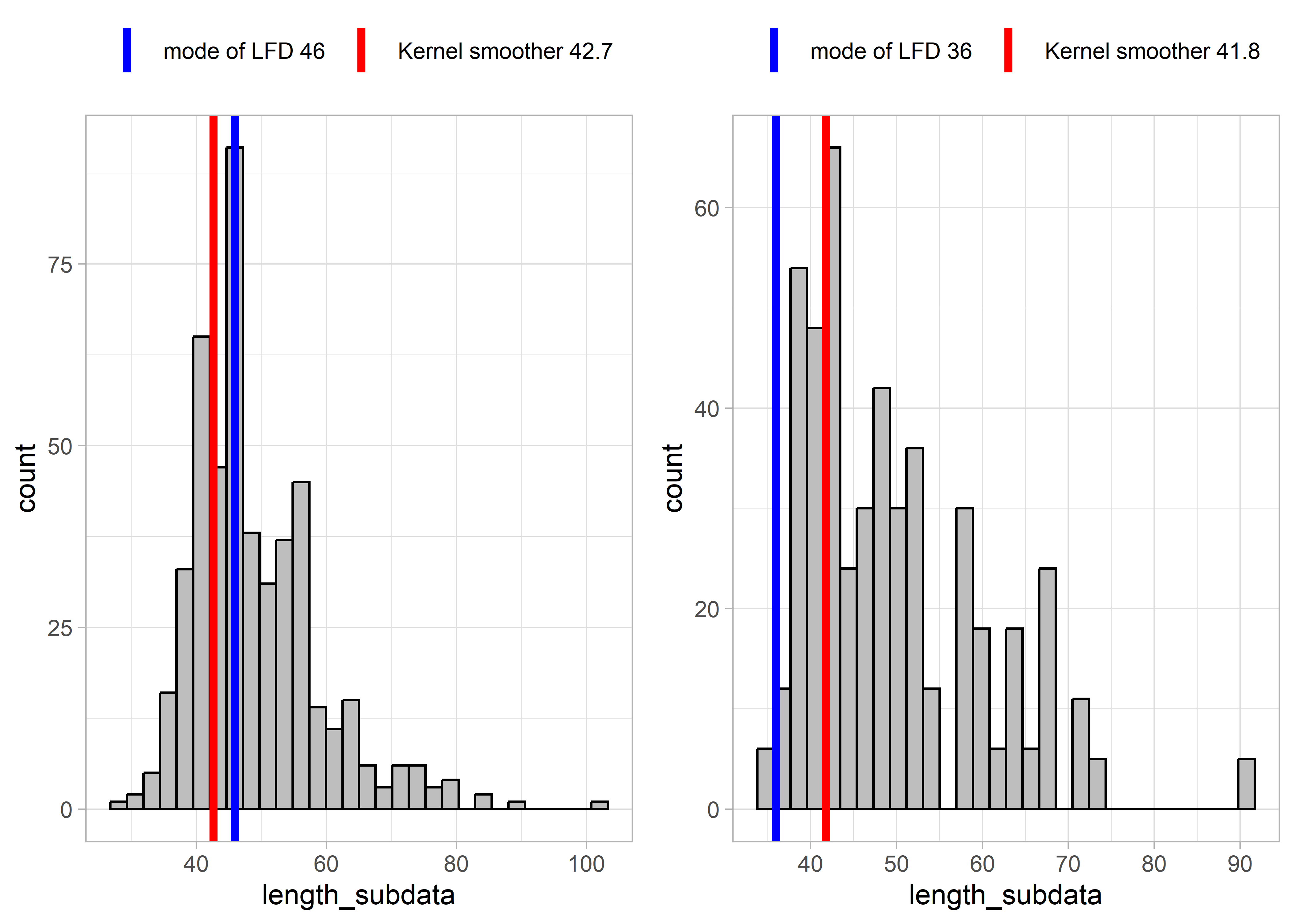
Figure 5.3: Example LFD 2019
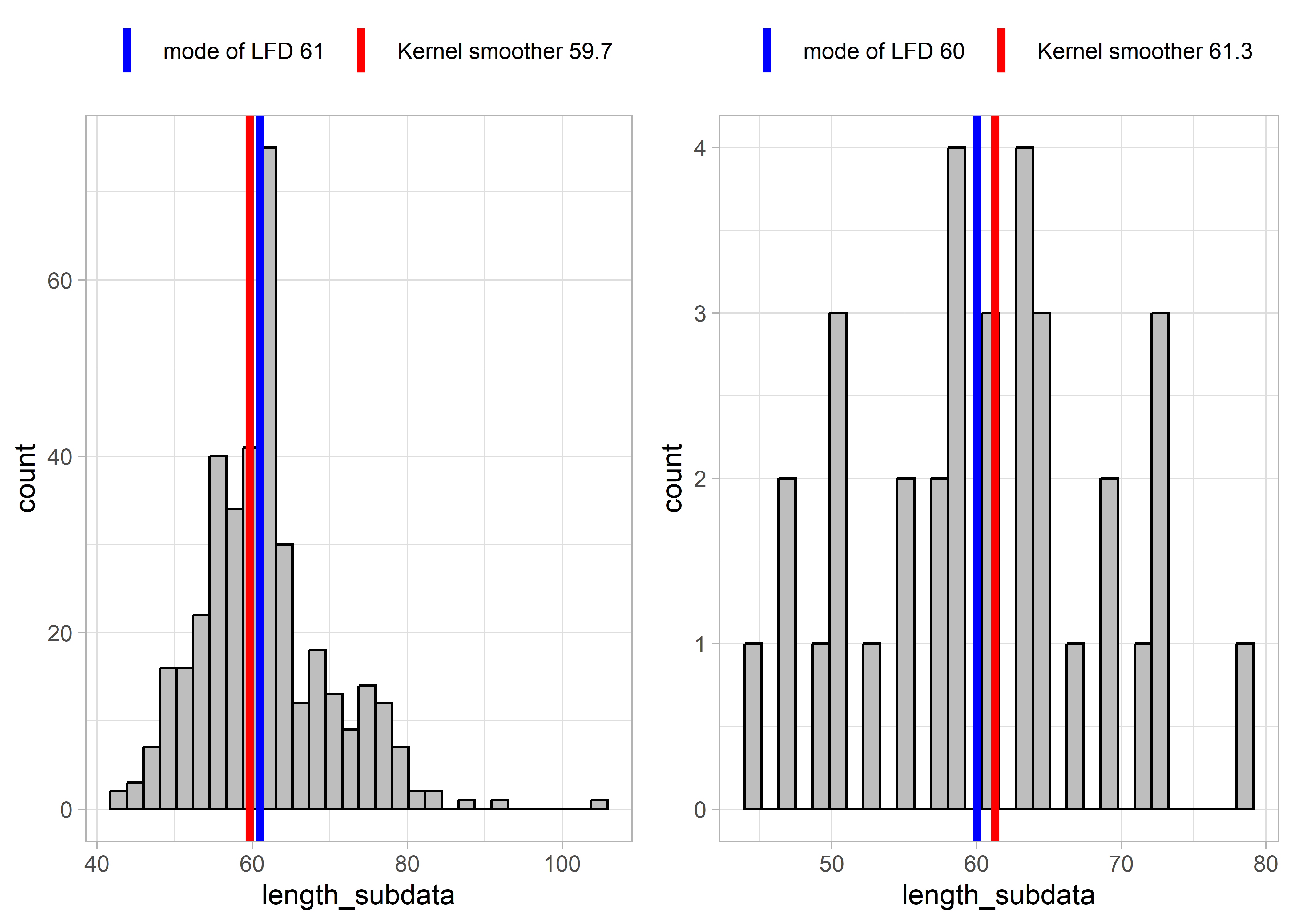
Figure 5.4: Example LFD 2018
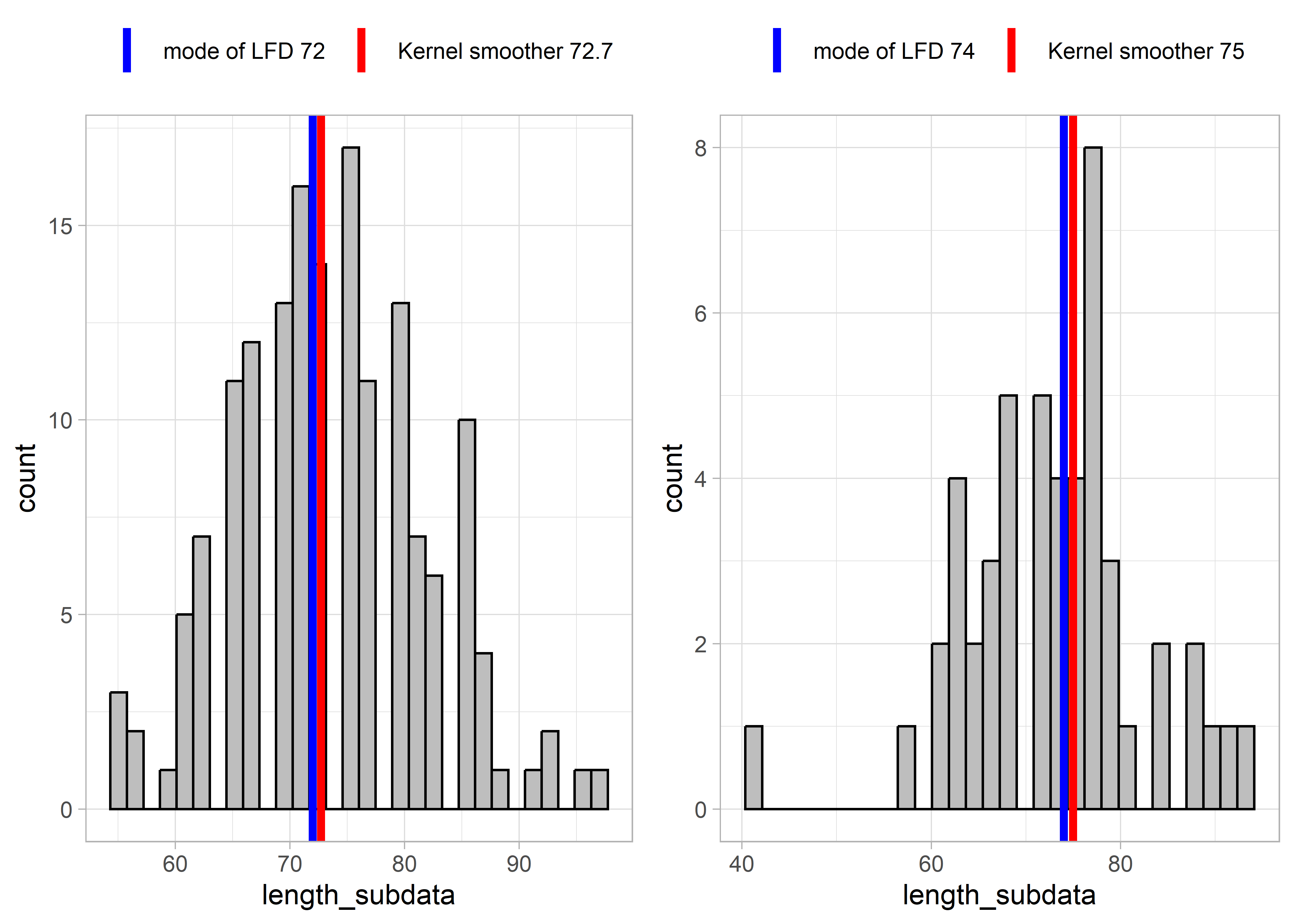
Figure 5.5: Example LFD 2015
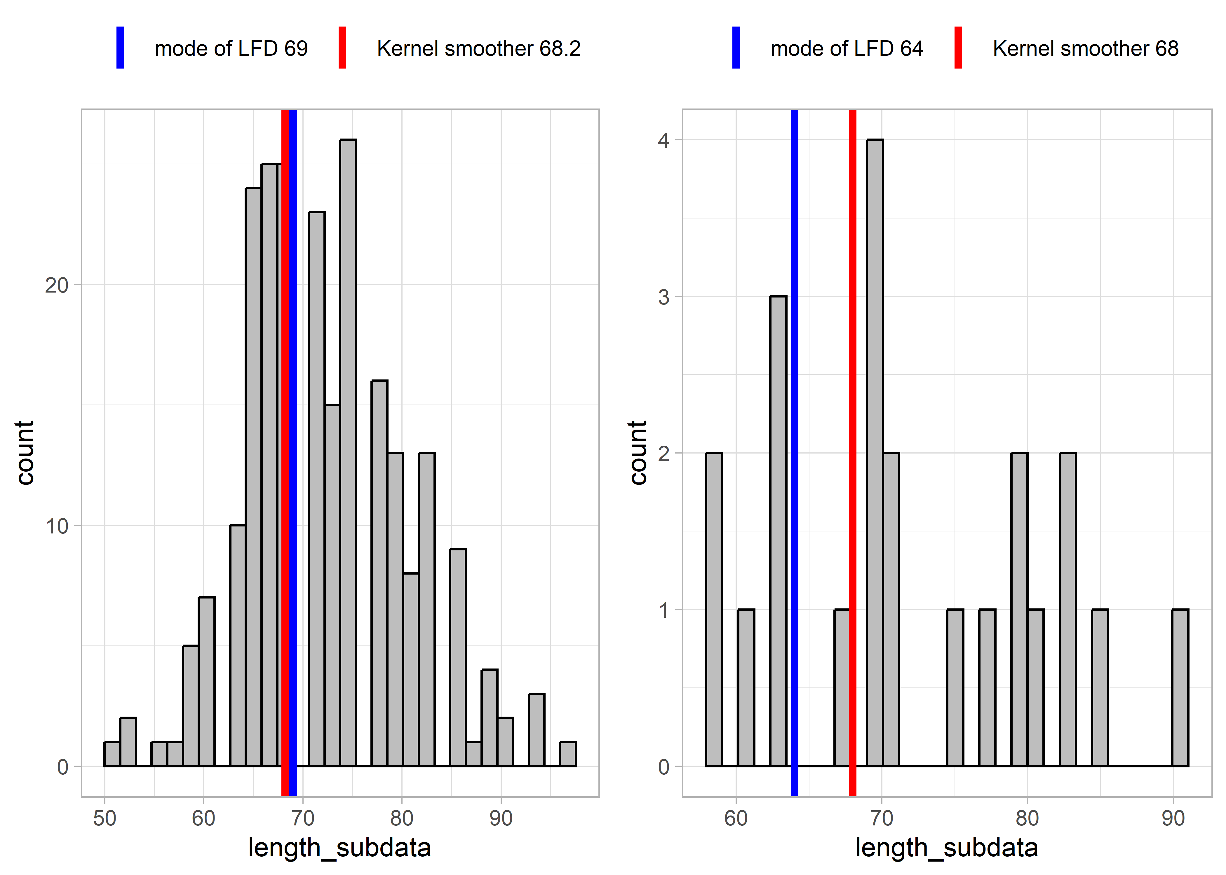
Figure 5.6: Example LFD 2017
These results show that for relatively complete LFDs (higher sample size, left-hand plots), the two methods (mode of LFD and kernel smoother) estimate similar lengths at full selectivity Lc. However, for more sparse length data (right-hand plots), the mode of the LFD might give very different results as for the example LFDs for 2019 and 2017. This is because the highest slope of the cumulative distribution occurred at smaller lengths. The kernel smoother seems to give more stable/reliable estimates of length at full selectivity.
5.4 fit_gillnet_dome function and gillnet selectivity analysis
Gillnets retain fish based on size selectivity, where the probability of retention varies with fish length and mesh size. To quantify this selectivity, statistical models (e.g., normal or lognormal curves) are fit to catch data collected across multiple mesh sizes. Each mesh size in a gillnet has its own retention curve, modeled using a probability function. The TropFishR package implements various models using the SELECT method of Russell Millar’s selectivity equations. So the the gillnet selectivity analysis presenetd here is built upon the theoretical framework developed by Millar and Holst (1997) for gillnet selectivity analysis and the modification to that framework made by Mildenberger, Taylor, and Wolff (2017).
This document describes the fit_gillnet_dome() function, which fits gillnet selectivity models using the TropFishR package. The function supports multiple dome-shaped selectivity models, and generates diagnostic plots. The fit_gillnet_dome() function is included as a standalone function in the R package fishLengthAssess.
The function fits five models to length-frequency data collected from gillnets with different mesh size. The mathematics behind this involves modeling how fish of different sizes are caught by different mesh sizes, accounting for the selectivity characteristics of each mesh. The deviance residuals and goodness-of-fit statistics are used to evaluate model performance.
The selectivity models include:
- norm.loc: Normal (common spread) model
- norm.sca: Normal (scaled spread) model
- lognorm: Lognormal model
- binorm.sca: Bi-normal model
- bilognorm: Bi-lognormal model
1. Normal Location Model (norm.loc)
The normal location model assumes that the selectivity follows a normal distribution with a fixed spread across mesh sizes. Assumes selectivity curves shift with mesh size but maintain the same spread (standard deviation:
\[S(L,m) = \exp\left(-\frac{(L - k \cdot m)^2}{2\sigma^2}\right)\]
Where \(S(L,m)\) is the is the selectivity at fish length L and mesh size m, \(k\) is a scaling parameter for the modal length (estimated), and \(\sigma\) is the standard deviation (spread of the curve).\(k\) and \(\sigma\) are estimated parameters.
2. Normal Scale Model (norm.sca)
This model also assumes a normal curve per mesh, but the spread (standard deviation) increases proportionally with mesh size. This model allows selectivity curves to have different widths depending on mesh size.
\[S(L,m) = \exp\left(-\frac{(L - k_1 \cdot m)^2}{2 \cdot k_2 \cdot m^2}\right)\]
Where \(k_1\) determines the modal length, and \(k_2\) controls how the standard deviation scales with mesh size. This model allows wider selectivity curves for larger meshes.\(k_1\) and \(k_2\) are estimated parameters.
3. Lognormal Model (lognorm)
The lognormal model assumes that the selectivity follows a lognormal distribution, which often provides a better fit for skewed length-frequency data. This model is commonly used when selectivity increases and decreases asymmetrically around the peak. Single peak, right-skewed.
\[S(L,m) = \frac{m}{L} \cdot \exp\left(\mu + \ln\left(\frac{m}{m_1}\right) - \frac{\sigma^2}{2}\right) \cdot \exp\left(-\frac{(\ln(L) - \mu - \ln\left(\frac{m}{m_1}\right))^2}{2\sigma^2}\right)\] Where \(\mu\) is the log-scale mean for the reference mesh size, \(\sigma\) is the log-scale standard deviation, and \(m_1\) is the reference mesh size (typically the smallest). \(\mu\) and \(\sigma\) are estimated parameters.
4. Bi-normal Scale Model (binorm.sca)
The bi-normal scale model combines two normal distributions, often representing different capture processes (e.g., wedging and tangling). Bi-normal distribution models two peaks in selectivity (if distinct Mode1 and Mode2), useful for species with two size classes that are selectively retained.
\[S(L,m) = p \cdot \exp\left(-\frac{(L - k_1 \cdot m)^2}{2 \cdot \sigma_1 \cdot m^2}\right) + (1-p) \cdot \exp\left(-\frac{(L - k_2 \cdot m)^2}{2 \cdot \sigma_2 \cdot m^2}\right)\]
Where \(p\) is the proportion of retention assigned to the first peak , \(k_1, k_2\) determine the modal lengths for each component, \(\sigma_1\) and \(\sigma_2\) control the standard deviations for each component. \(p\) is calculated as:
\[ p = \frac{\exp(\theta)}{1 + \exp(\theta)} \] The estimated parameters in the bi-normal scale model are: \(k_1\) and \(k_2\), \(\sigma_1\) and \(\sigma_2\), and \(\theta\). \(\theta\) is estimated in logit scale and \(p\) is its inverse logit, therefore the final estimate of \(p\) is always between 0 and 1 (a valid probability)
5. Bi-lognormal Model (bilognorm)
The bi-lognormal model combines two lognormal distributions and captures two peaks (if distinct Mode1 and Mode2) but with lognormal-based selectivity functions, allowing for asymmetric selectivity at both peaks. The selectivity-at-length function for mesh size \(m\) is given by:
\[ S(L, m) = p \cdot \left( \frac{m}{L} \right) \cdot \exp\left( \mu_1 + \ln\left(\frac{m}{m_1}\right) - \frac{\sigma_1^2}{2} \right) \cdot \exp\left( -\frac{ \left( \ln(L) - \mu_1 - \ln\left(\frac{m}{m_1}\right) \right)^2 }{2 \sigma_1^2} \right) + (1 - p) \cdot \left( \frac{m}{L} \right) \cdot \exp\left( \mu_2 + \ln\left(\frac{m}{m_1}\right) - \frac{\sigma_2^2}{2} \right) \cdot \exp\left( -\frac{ \left( \ln(L) - \mu_2 - \ln\left(\frac{m}{m_1}\right) \right)^2 }{2 \sigma_2^2} \right) \]
Where \(m_1\) is the reference mesh size (usually the smallest in the set), \(\mu_1\) and \(\mu_2\) are the log-scale location parameters for the two domes, \(\sigma_1\) and \(\sigma_2\) are the log-scale spread parameters for the two domes, and \(p\) is the proportion of fish following the first dome (proportion of retention assigned to the first peak), estimated as:
\[ p = \frac{\exp(\theta_5)}{1 + \exp(\theta_5)} \] The estimated parameters in the bi-lognormal model are: \(\mu_1\), \(\mu_2\), \(\sigma_1\) and \(\sigma_2\) in log-scale. \(\theta\) is estimated in logit scale and \(p\) is its inverse logit, therefore the final estimate of \(p\) is always between 0 and 1 (a valid probability).
5.4.1 Function Overview
The fit_gillnet_dome is part of the fishLengthAssess R package and the function contains the following key features:
The function allows the user to decide whether to fit all five models (i.e., norm.loc, norm.sca, lognorm, binorm.sca and bilognorm) or to omit the bimodal models (binorm.sca and bilognorm), using the arument
run_bimodal=FALSE/TRUE. By default, the bimodal models are omitted (FALSE).Generates selectivity curves and residual plots for each model.
Provides statistics to compare model performance.
It automatically calculates appropriate starting values for complex selectivity models (e.g., binorm.sca and bilognorm) based on the length distribution of data.
Also, it allows the user to use pre-defined starting values when automatic calculation for binorm.sca and bilognorm is suboptimal.
Creates diagnostic plots to understand length distributions across mesh sizes. The
fit_gillnet_dome()function streamlines the workflow of gillnet selectivity analysis through three main steps:Exploratory analysis and automatic starting value estimation
Model fitting for multiple selectivity curves
Result visualization and comparative statistics
5.4.2 Function Arguments
| Arguments | Description |
|---|---|
input_data |
Data frame with fish lengths in first column and catches for each mesh size in subsequent columns |
mesh_sizes |
Vector of mesh sizes in the same order as the columns in input_data |
run_bimodal |
Logical (TRUE/FALSE) that controls whether bimodal models (binorm.sca and bilognorm) are fitted. Default: FALSE |
manual_x0_list |
Optional list of manually specified starting values for each model type |
length_seq |
Sequence of length values for plotting selectivity curves (default: 40-100 cm by 0.1) |
output_dir |
Directory where plots will be saved (default: “model_plots”) |
criterion |
Criterion for model selection (“Deviance” or “LogLikelihood”) |
sd_spread |
Range around detected modes used to calculate starting values for standard deviations (default: 7) |
rel.power |
Optional vector of relative fishing powers for each mesh size |
verbose |
Whether to print progress messages (default: TRUE) |
5.4.3 Data exploration and calculation of starting values
The first step of the function performs exploratory analysis to understand the catch distribution across length classes and mesh sizes. It then uses these insights to automatically calculate appropriate starting values for the optimization process.
Data visualization
Four key plots are generated and saved in the specified output directory:
- Length distribution by mesh size: Histograms showing catch at each length class for each mesh.
- Catch distribution across length classes: Line plots comparing catch patterns between mesh sizes.
- Aggregated length distribution: Bar plot of total catch by length class across all meshes.
- Detected peaks: Visualization of the identified modes in the length frequency data.
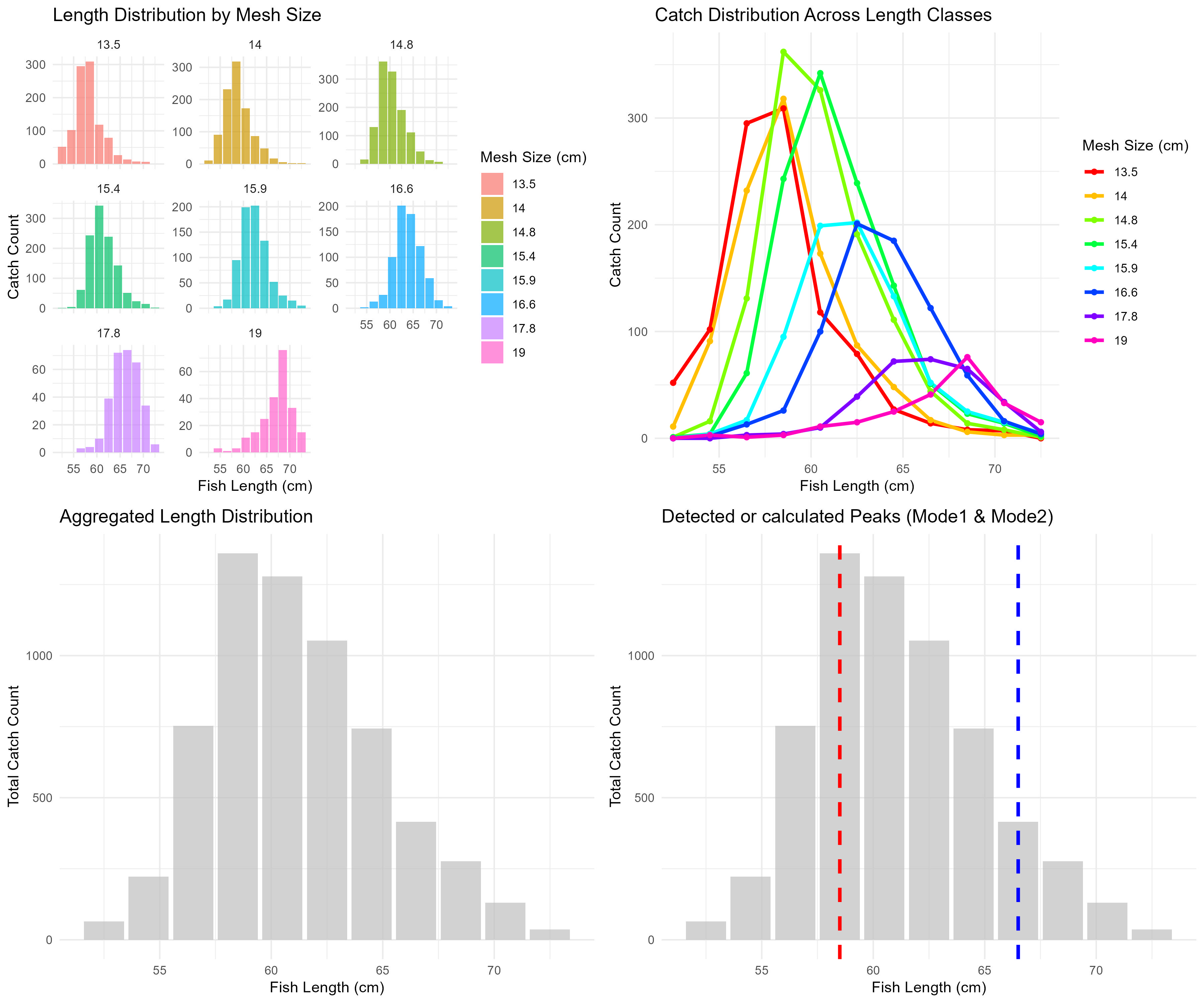
Figure 5.7: Exploratory visualization of data.
The above plot shows the four exploratory visualizations combined. The first panel (top left) shows the length distribution by mesh size, the second panel (top right) shows the catch distribution across length classes, the third panel (bottom left) shows the aggregated length distribution, and the fourth panel (bottom right) shows the detected peaks (Mode1 in red, Mode2 in blue).
Calculation of starting values for binorm.sca and bilognorm
An important feature of this function is that it only calculates and provides starting values (x0) for the more complex bimodal models (binorm.sca and bilognorm). For the simpler models (norm.loc, norm.sca, and lognorm), x0 is intentionally set to NULL. This is because:
The select_Millar() function internally calls gillnetfit() for these simpler models, which has its own robust mechanism for estimating initial values.
Simpler models are less sensitive to starting values and generally converge well without external initialization.
Bimodal models have more parameters (including the proportion parameter p) and are more prone to convergence issues without good starting values.
The function uses the findpeaks() function from the pracma package to detect modes in the aggregated length distribution:
nups = 2: Requires at least 2 increasing points before the peakndowns = 2: Requires at least 2 decreasing points after the peakminpeakheight = max(total_counts) * 0.1: Ignores small peaks (less than 10% of maximum)
Starting values calculation
The function handles three scenarios:
- Two or more peaks detected:
- Mode1 = location of first peak
- Mode2 = location of second peak
- Only one peak detected:
- Mode1 = location of the peak
- Mode2 = location of highest catch at least 5 cm away from Mode1, or 75th percentile if no suitable secondary peak
- No clear peaks:
- Mode1 = 30th percentile of length distribution
- Mode2 = 70th percentile of length distribution
Standard deviations are estimated from the data in windows around each mode:
#It keeps all lengths within a window of +/- sd_spread cm around Mode1 and Mode2.
#e.g. if Mode1 = 40 and sd_spread = 7, it keeps lengths from 33 to 47 cm

subset1 <- plot_data$MidLength[plot_data$MidLength > (Mode1 - sd_spread) & plot_data$MidLength < (Mode1 + sd_spread)] #selects a subset of fish lengths around Mode1

subset2 <- plot_data$MidLength[plot_data$MidLength > (Mode2 - sd_spread) & plot_data$MidLength < (Mode2 + sd_spread)] #selects a subset of fish lengths around Mode2

#Now if If the SD is missing (NA), or too small (less than 3 cm) (too narrow curve). Then it defaults to 3.5 cm as a safe minimum value
StdDev1 <- ifelse(is.na(sd(subset1)) || sd(subset1) < 3, 3.5, sd(subset1))
StdDev2 <- ifelse(is.na(sd(subset2)) || sd(subset2) < 3, 4.5, sd(subset2))
For bimodal models, the function also calculates the proportion parameter based on the relative catch in each mode:
Catch_Mode1 <- sum(total_counts[plot_data$MidLength > (Mode1 - sd_spread) &
                                plot_data$MidLength < (Mode1 + sd_spread)], na.rm = TRUE)
Catch_Mode2 <- sum(total_counts[plot_data$MidLength > (Mode2 - sd_spread) &
                                plot_data$MidLength < (Mode2 + sd_spread)], na.rm = TRUE)
P_Mode1 <- min(max(Catch_Mode1 / (Catch_Mode1 + Catch_Mode2), 0.75), 0.95)
P_Mode1_logit <- qlogis(P_Mode1)  # Convert to logit scale
For lognormal-based models, the function converts raw-space parameters to log-space parameters:
log_sd_from_raw <- function(mean_val, sd_val) sqrt(log(1 + (sd_val / mean_val)^2))
LogStdDev1 <- min(max(log_sd_from_raw(Mode1, StdDev1), 0.1), 0.4)
LogStdDev2 <- min(max(log_sd_from_raw(Mode2, StdDev2), 0.1), 0.4)
This transformation uses the mathematical relationship between normal and lognormal distributions:
If \(X \sim \text{LogNormal}(\mu, \sigma^2)\), then: - Mode of \(X = e^{\mu - \sigma^2}\) - Variance of \(X = (e^{\sigma^2} - 1) \cdot e^{2\mu + \sigma^2}\)
Solving for \(\sigma\) given the mode and standard deviation: \(\sigma = \sqrt{\log\left(1 + \left(\frac{\text{StdDev}}{\text{Mode}}\right)^2\right)}\)
5.4.4 Model Fitting
This step fits multiple selectivity models using the automatically calculated starting values from the previous step or using starting values manually provided if specified.
The run_bimodal parameter controls which models are fitted:
When run_bimodal = TRUE (default): All five selectivity models are fitted (three unimodal and two bimodal models)
When run_bimodal = FALSE: Only the three unimodal models are fitted.
| Category | Models | Description |
|---|---|---|
| Unimodal | norm.loc, norm.sca, lognorm |
Always fitted regardless of run_bimodal setting |
| Bimodal | binorm.sca, bilognorm |
Only fitted when run_bimodal = TRUE |
The function fit_gillnet_dome prepares the data in the format required by the select_Millar() function:
data_list <- list(
  midLengths = midLengths,
  meshSizes = mesh_sizes,
  CatchPerNet_mat = CatchPerNet_mat,
  rel.power = rel.power
)
In the model fitting loop, three or five models are fitted:
- Normal location (norm.loc)
- Normal scale (norm.sca)
- Lognormal (lognorm)
- Bi-normal scale (binorm.sca) (optional)
- Bi-lognormal (bilognorm) (optional)
Each model in the selected set is fitted sequentially using an error-handling approach:
for (model in models) {
  cat("\nFitting model:", model, "...\n")

  # Determine starting values for each model
  x0 <- if (model %in% names(full_x0_list)) full_x0_list[[model]] else NULL

  # Try to fit the model, catch any errors
  results[[model]] <- tryCatch({
    select_Millar(data_list, x0 = x0, rtype = model, rel.power = rel.power, plot = FALSE)
  }, error = function(e) {
    cat("Error fitting model:", model, "- Skipping.\n")
    return(NULL)
  })
}

results <- results[!sapply(results, is.null)]
  if (length(results) == 0) {
    cat("No models fitted successfully.\n")
    return(NULL)
  }
This loop iterates through each model type (unimodal and bimodal if selected),provides informative output to track progress during model fitting, and determines appropriate starting values:
- For bimodal models: Uses the automatically detected peaks or manually provided values.
- For unimodal models: Allows the
select_Millar()function to calculate starting values internally.
Also, the loops contains a tryCatch() to handling errors:
- If a model successfully fits: Stores the result in the results list.
- If a model fails to converge or encounters numerical issues: Captures the error, logs a message, and continues with the next model. This prevents a single problematic model from causing the entire analysis to fail.
After the loop completes, the function filters out any failed models before proceeding to model comparison and visualization steps.
5.4.5 Model parameter summary
After fitting, a summary table is created with key parameters from each model:
summary_table <- data.frame(
  Model = names(results),
  LogLikelihood = sapply(results, function(x) x$out["model.l", 1]),
  Deviance = sapply(results, function(x) x$out["Deviance", 1]),
  Mode1 = sapply(results, function(x) x$estimates[1, "par"]),
  StdDev1 = sapply(results, function(x) x$estimates[2, "par"]),
  Mode2 = sapply(results, function(x) ifelse(nrow(x$estimates) > 2, x$estimates[3, "par"], NA)),
  StdDev2 = sapply(results, function(x) ifelse(nrow(x$estimates) > 3, x$estimates[4, "par"], NA)),
  P_Mode1 = sapply(results, function(x) ifelse(nrow(x$estimates) > 4, x$estimates[5, "par"], NA))
)
Models are sorted by Deviance and Log-likelihood values. Log-Likelihood and Deviance are statistical measures used to evaluate the goodness of fit of different models. The Log-Likelihood value indicates how well a model fits the observed data. Higher values are better (closer to zero, as log-likelihoods are negative). When comparing models with the same number of parameters, the one with the higher log-likelihood provides a better fit.
Deviance is derived from the log-likelihood and measures the departure of the model from a perfectly fitting model. It allows for formal statistical tests between nested models. The model with the lowest deviance provides the closest fit to the observed data.
Based on the Log-likelihood values, the user can calculate AIC (AIC = -2 × log-likelihood + 2 × k), where k is the number of parameters. The model with the lowest AIC is considered the best balance between goodness-of-fit and parsimony.
The following table shows an example of a statistical summary.
| Model | LogLikelihood | Deviance | Mode1 | StdDev1 |
|---|---|---|---|---|
| lognorm | 25014.23 | 704.28 | 54.91 | 4.46 |
| norm.sca | 24979.99 | 772.76 | 55.28 | 4.34 |
| norm.loc | 24934.91 | 862.92 | 54.60 | 5.15 |
5.4.6 Result visualization and interpretation
The final step creates visual outputs for each successfully fitted model.
Selectivity curves
For each model, selectivity curves are calculated for all mesh sizes across the specified length range:
rmatrix <- outer(plotlens, meshSizes, rtypes_Millar(res$rtype), res$par)
rmatrix <- t(t(rmatrix) * res$rel.power)
These curves show the relative retention probability for fish of different lengths in each mesh size.
Deviance Residuals
Deviance residuals help assess model fit by showing where the model predictions differ from observed data:
dev_res_df <- data.frame(
  Length = rep(res$midLengths, times = nmeshes),
  MeshSize = factor(rep(meshSizes, each = length(res$midLengths))),
  Residuals = as.vector(res$Dev.resids)
)
Bubble plots visualize these residuals, with: - Bubble size proportional to residual magnitude - Blue bubbles for negative residuals (model overprediction) - Red bubbles for positive residuals (model underprediction)
Output plots
For each model, the function creates and saves: 1. A selectivity curve plot showing relative retention by length for each mesh size 2. A deviance residual bubble plot showing fit quality across lengths and mesh sizes 3. Combined plots with both visualizations together
Below are two examples of plots for two different selectivity models:
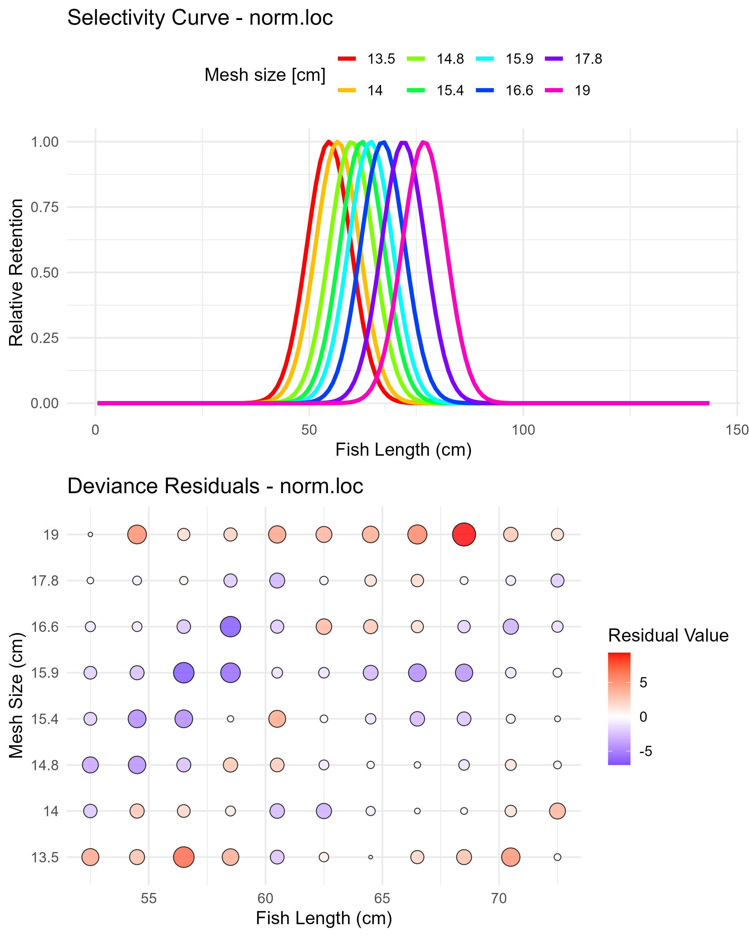
Figure 5.8: Normal location model (norm.loc) selectivity curves and residuals. The top panel shows the selectivity curves for each mesh size, while the bottom panel displays the deviance residuals.
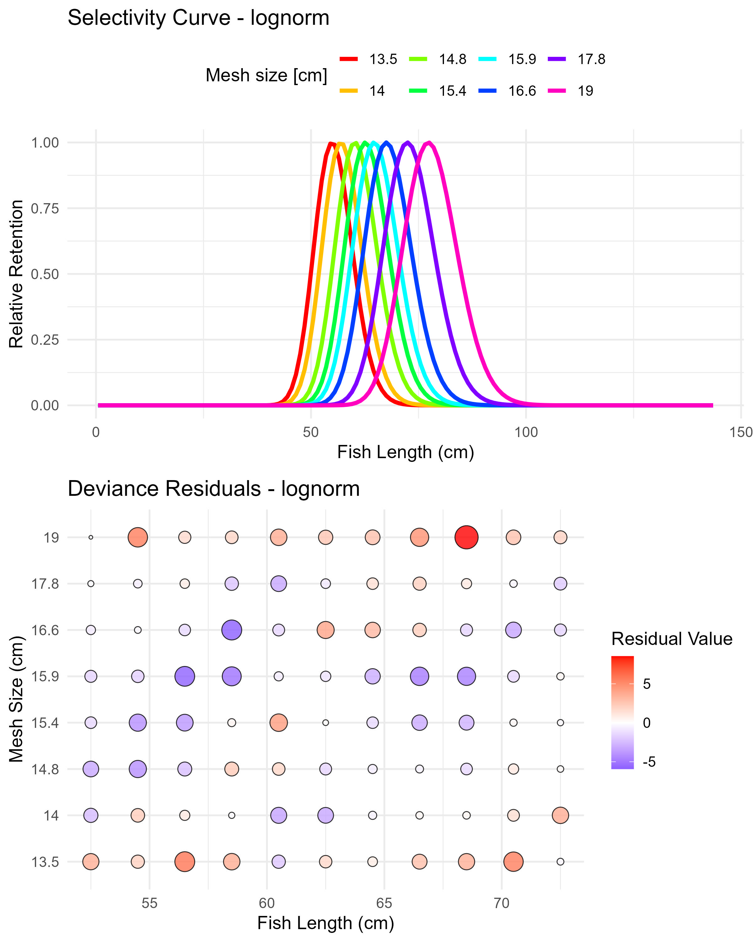
Figure 5.9: Lognormal model (lognorm) selectivity curves and residuals. The top panel shows the selectivity curves for each mesh size, while the bottom panel displays the deviance residuals.
Each plot shows:
- Selectivity curve plot (top panel):
- X-axis: Fish length (cm)
- Y-axis: Relative retention (scaled to maximum of 1)
- Lines: Each colored line represents a different mesh size
- Interpretation:
- Each curve shows the relative probability of catching fish of different lengths with a specific mesh size
- The peak of each curve indicates the optimal fish length for that mesh size
- Curves typically shift to the right as mesh size increases
- The width of curves indicates the selectivity range
- Comparing curve shapes across models helps evaluate which provides the most realistic representation
- Deviance residuals bubble plot (bottom panel)
- X-axis: Fish length (cm)
- Y-axis: Mesh size (cm)
- Bubbles:
- Size: Indicates the absolute magnitude of the deviance residual
- Color: Blue for negative residuals (model overestimates), red for positive residuals (model underestimates)
- Position: Each bubble positioned at specific length × mesh size combination
- Interpretation:
- Good-fitting models have smaller bubbles distributed randomly
- Systematic patterns (e.g., clusters of same-colored bubbles) indicate areas where the model fits poorly
- Areas with large bubbles indicate specific length-mesh combinations where the model predictions differ substantially from observed data
These visualizations are saved for each model in the specified output directory, providing a comprehensive visual assessment of model performance.
In Chapter 6, the user will find a a complete example showing how to use the fit_gillnet_dome function with real data (See section 6.1 for details).