8 Examples
8.1 Projection modeling
This example demonstrates implementation of Projection Modeling. Projection modeling differs from an MP in that projections consist of ‘static’ actions such as a size limit or constant fishing effort, whereas MPs are ‘dynamic’ responses to updated information (e.g., pre-agreed responses to observations of the fishery system). While making such projections are strictly speaking not the same MPs, setting up projection modeling follows the same coding in FishSimGTG and relies on specification of a StrategyObj.
Below, a complex OM is defined with three areas. Projection modeling is used to evaluate a suite of management options, including size limits, effort reductions (such as seasonal closures or time-day closures). All projections are developed under the assumption that fishing effort is re-allocated from closed areas to open areas, rather than being removed from the fishery.
8.1.1 Populate the life history object
See Section 3 for details on how to populate the Operating Model.
LifeHistoryObj <- new("LifeHistory")
LifeHistoryObj@title<-"Honeycomb grouper"
LifeHistoryObj@speciesName<-"EpinephelusMerra"
LifeHistoryObj@shortDescription<-"example multiple areas"
LifeHistoryObj@Linf<-24.4
LifeHistoryObj@K<-0.2
LifeHistoryObj@t0<- 0
LifeHistoryObj@L50<-14.1
LifeHistoryObj@L95delta<-2.1
LifeHistoryObj@M<-0.29
LifeHistoryObj@L_type<-"FL"
LifeHistoryObj@L_units<-"cm"
LifeHistoryObj@LW_A<-0.016
LifeHistoryObj@LW_B<-2.966
LifeHistoryObj@Walpha_units<-"g"
LifeHistoryObj@Steep<-0.69
LifeHistoryObj@recSD<-0.6
LifeHistoryObj@recRho<-0
LifeHistoryObj@isHermaph<-FALSE #ignored for demo purposes
LifeHistoryObj@R0<-10000
8.1.2 Populate the historical fishery object
This structure assumes a fishery operating during the historical time with same fishery characteristics in each area.
8.1.3 Populate the time-area object
The three areas are specified to recieve approximately equal numbers of recruits. The historical dynamics are simulated to reflect an initial depletion level of 0.5, followed by a stable level of fishing effort for 10 years.
# I want to run the low movement scenario
TimeAreaObj<-new("TimeArea")
TimeAreaObj@title <- "Test"
TimeAreaObj@gtg <- 13
TimeAreaObj@areas <- 3
TimeAreaObj@recArea <- c(0.33, 0.33,0.34)
TimeAreaObj@iterations <- 100
TimeAreaObj@historicalYears <- 10
TimeAreaObj@historicalBio <- 0.5
TimeAreaObj@historicalBioType <- "relB"
TimeAreaObj@move <- matrix(c(
  0.9, 0.05, 0.05,
  0.05, 0.9, 0.05,
  0.05, 0.05, 0.9), nrow=3, ncol=3, byrow=TRUE)
TimeAreaObj@historicalEffort <- matrix(1:1, nrow = 50, ncol = 3, byrow = FALSE)
The slot TimeAreaObj@move defines the proportion of abundance migrating to other areas. Columns are ‘from area’ and rows are ‘to area’.
#E.g. A two-area model:
#        [,1]                     [,2]
# [1,]   Area 1 staying in 1      Area 2 going to 1
# [,2]   Area 1 going to 2        Area 2 statying in 2

#To specify no movement in a two-area model, use:
matrix(c(1,0, 0,1), nrow=2, ncol=2, byrow=FALSE)
## [,1] [,2]
## [1,] 1 0
## [2,] 0 1In the current example, 90% of individuals do not change areas annually, with 5% going to each of the other two adjacent areas.
##      [,1] [,2] [,3]
## [1,] 0.90 0.05 0.05
## [2,] 0.05 0.90 0.05
## [3,] 0.05 0.05 0.90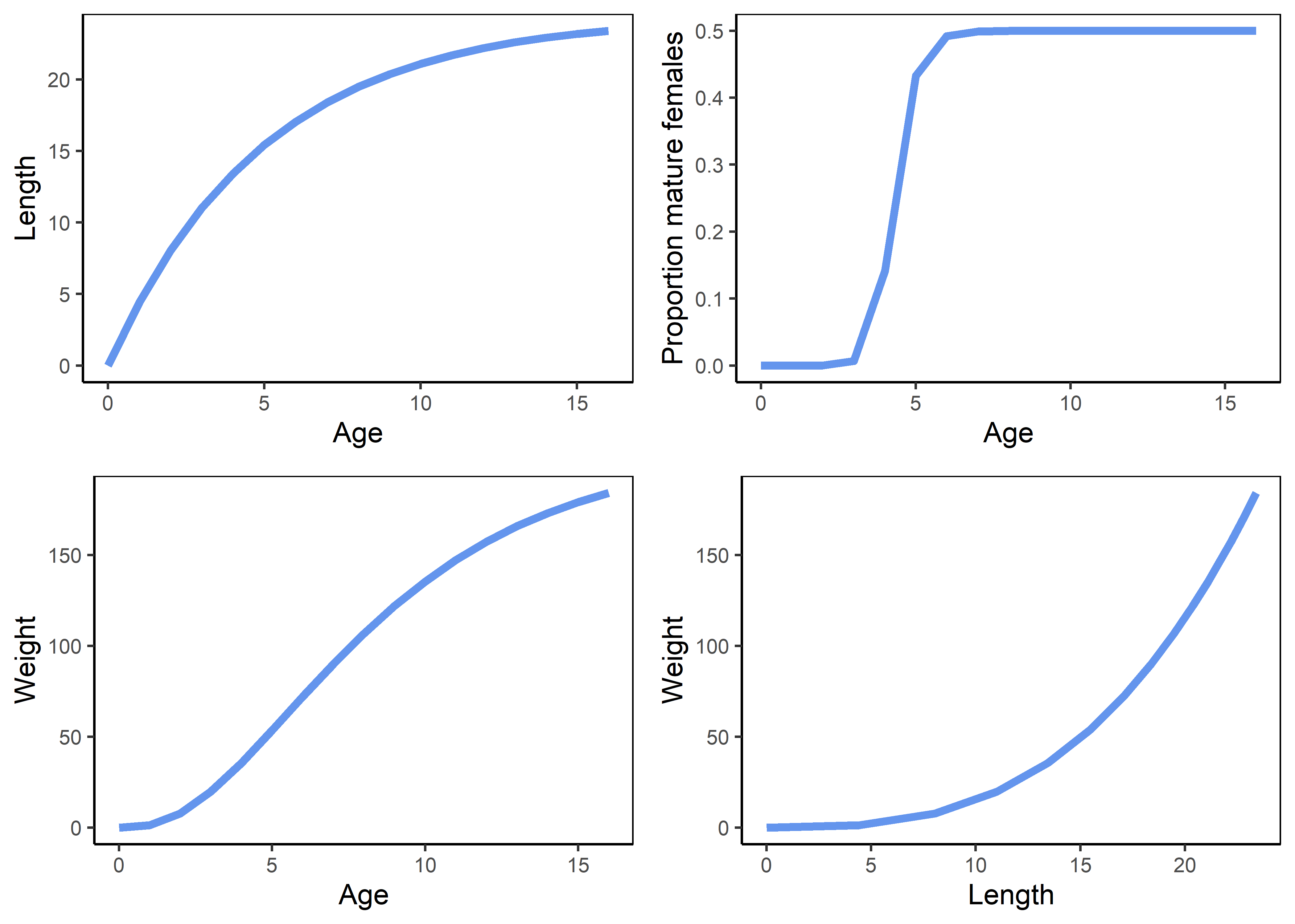
8.1.6 Include uncertainty
In this example, uniform distributions are specified to reflect uncertainty in life history and historical fishery vulnerability.
StochasticObj<-new("Stochastic")
StochasticObj@historicalBio <- c(0.2, 0.6)
StochasticObj@Linf <- c(24.4, 29.8)
StochasticObj@K <- c(0.2, 0.97)
StochasticObj@L50 <- c(14.1, 16.8)
StochasticObj@L95delta <- c(2.1, 2.5)
StochasticObj@M <- c(0.29, 0.43)
StochasticObj@Steep <- c(0.69, 0.84)
StochasticObj@histFisheryVul <- matrix(c(10,14,0.5,1), nrow=2, ncol=2,byrow=FALSE)
StochasticObj@sameFisheryVul <- TRUE
In the HistFisheryObj, HistFisheryObj@vulType<-"logistic", thus requiring two input parameters to describe the logistic vulnerability function. To introduce uncertainty into these two parameters, a 2 x 2 matrix is required with columns reflecting number of parameters and rows representing minimum and maximum values for each parameter.
##      [,1] [,2]
## [1,]   10  0.5
## [2,]   14  1.0
8.1.7 Specify projection conditions
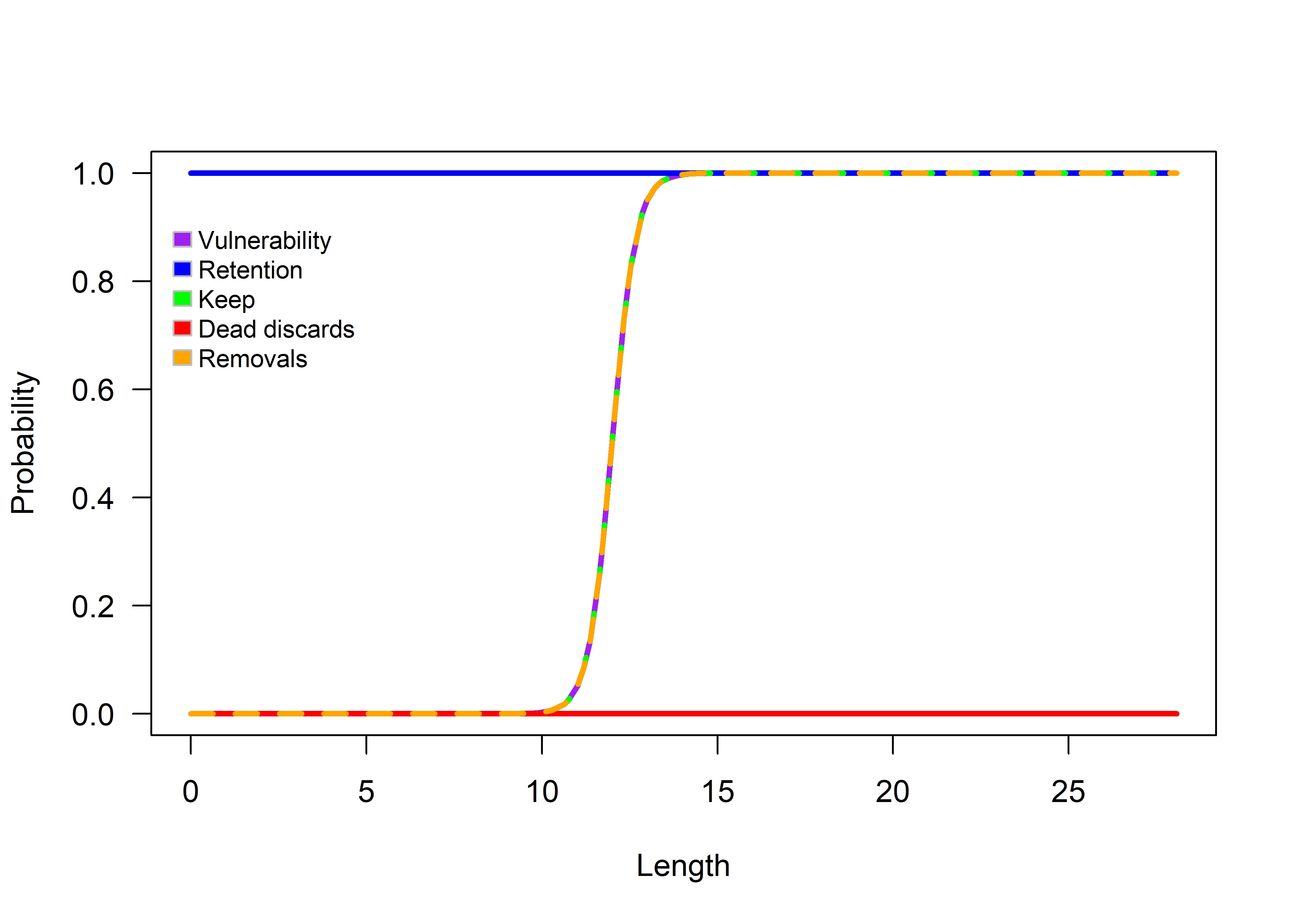
Like defining an MP, projection modeling requires two additional S4 objects are needed: ProFisheryObj and StrategyObj. The forward projection fishery object is specified to implement a size limit of 14 cm (see ProFisheryObj@retType and ProFisheryObj@retParams). Notice that StochasticObj@sameFisheryVul=TRUE, so the uncertainty range for vulnerability in the historical time period will also be applied to the projection time period, ignoring ProFisheryObj@vulType and ProFisheryObj@vulParams. Thus, in this example, fishery selectivity is consistent between historical and projection time periods, but a size limit is implemented by modifying retention (and correspondingly assuming discard mortality is zero ProFisheryObj@Dmort <- 0).
ProFisheryObj <- new("Fishery")
ProFisheryObj@title <- "Test"
ProFisheryObj@vulType <- "logistic"
ProFisheryObj@vulParams <- c(12, 1)
ProFisheryObj@retType <- "logistic"
ProFisheryObj@retParams <- c(14, 0.1)
ProFisheryObj@retMax <- 1
ProFisheryObj@Dmort <- 0

#Finally, we need to define fishery characteristics for each area in the OM.
#In this case, we will assume each area has the same fishery characteristics
ProFisheryObj_list <- list(ProFisheryObj, ProFisheryObj, ProFisheryObj)
The second additional object is the StrategyObj. The built in MP named projectionStrategy contains a variety of controls of static changes to fishery management, including control of fishing effort. The strategy considered is to close one area permanently and assume effort from the closed area will be dispersed equally to the remain two areas.
See MP library in section 5.4 for details
8.1.8 Running projections
runProjection(
  LifeHistoryObj = LifeHistoryObj,
  TimeAreaObj = TimeAreaObj,
  HistFisheryObj = HistFisheryObj,
  ProFisheryObj_list = ProFisheryObj_list,
  StrategyObj = StrategyObj,
  StochasticObj = StochasticObj,
  wd = here("data-test", "Kole"),
  fileName = "Size_option1",
  doPlot = TRUE,
  titleStrategy = "Min size 14 cm"
)
Next, we present some of the diagnostic plots produced by runProjection().