4 Management Procedures (MPs)
A Management Procedure (MP) is a pre-agreed process defining how a fishery will be managed, with the primary role being to take fishery information and return a management recommendation. One of the most distinctive features of FishSimGTG is that it allows the user to create customized MPs.
The FishSimGTG package can be used to make forward-projections for a variety of fishery management actions. Making forward projections requires the following set of S4-type objects. As previously discussed, the OM is comprised of three required objects in S4 format:
- Life history object (
LifeHistoryObj) - Historical fishery object (
HistFisheryObj) - Time-area object (
TimeAreaObj)
With optional:
- Stochastic object (
StochasticObj)
And, producing forward-simulation requires two additional objects in S4 format:
- Management procedure or harvest strategy object (
StrategyObj) - Projection time period fishery object (
ProFisheryObj)
4.1 Strategy object
The StrategyObj holds a set of instructions about how the fishery will be managed.
To create a new object of class StrategyObj, use the new() function.
The user can see the elements or slots of the StrategyObj using the slotNames() function.
## [1] "title" "projectionYears" "projectionName" "projectionParams"To populate the StrategyObj, the user should start by specifying a title (title) and the number of forward projection years to simulate (projectionYears).
The projectionName is a string that directs to a named function that contains a set of instructions about how the fishery will be managed. And, projectionParams is a list of input parameters that follows the specifications of the projection function defined in projectionName.
Developing the necessary code to create a custom StrategyObj can be very challenging. A StrategyObj can take the form of a simple projections or an MP. A simple projection differs from an MP in that projections consist of ‘static’ actions such as a size limit or constant fishing effort, whereas MPs are ‘dynamic’ actions such as annual adjustments to catch limits. MPs tend to be more complicated because they include a harvest control rule or decision-rule that is informed by updated information gathered from monitoring.
In subsequent sections of this chapter, we will build example MPs. The user is advised to first explore Projection Modeling, in which simple projections are demonstrated using built-in functions. Understanding simple projections is a useful pre-cursor to understanding how to design and implement code for more complex MPs.
4.2 Projection fishery object
The ProFisheryObj is an S4 object of the class Fishery that holds fishery characteristics, including vulnerability, retention, and discard information. Note that both the HistFisheryObj and
ProFisheryObj utilize the same S4 object class.
HistFisheryObj and ProFisheryObj are both Fishery objects. When no changes in the fishery characteristics are anticipated, the slots of ProFisheryObj can be set to the same values as those in HistFisheryObj
Alternatively, the user has the option to modify the HistFisheryObj object when performing fishery projections. These modifications are stored in a new ProFisheryObj.
To create a new object of class Fishery, use the new() function, as follows:
The slot names of the ProFisheryObj can be seen using the slotNames() function.
## [1] "title"     "vulType"   "vulParams" "retType"   "retParams" "retMax"
## [7] "Dmort"
The user can access the help file using ? symbol
ProFisheryObj can be populated as follows:
ProFisheryObj@title<-"Test"
ProFisheryObj@vulType<-"logistic"
ProFisheryObj@vulParams<-c(10.2,0.1)
ProFisheryObj@retType<-"logistic"
ProFisheryObj@retParams <- c(15, 0.1)
ProFisheryObj@retMax <- 1
ProFisheryObj@Dmort <- 0
In this example, during the projections, we maintain the same vulnerability type and parameters as in the HistFisheryObj object but modify retention to follow a logistic function.
4.2.2 Uncertainty in the projection fishery
Additional slots in the StochasticObj object allow for modifications to the fishery projection object. These additional slots, proFisheryVul_list, proFisheryRet_list, and proFisheryDmort_list, are lists where the number of list items corresponds to the number of areas (TimeAreaObj@areas). Each item in the list is a matrix with \(n\) columns and 2 rows, where the rows represent the minimum and maximum values for the parameters associated with each column \(n\).
When provided, these lists replace the vulParams, retParams, and Dmort slots in the fishery projections (ProFisheryObj). For proFisheryVul_list and proFisheryRet_list, the number of columns in the matrix align with the required inputs for ProFisheryObj@vulType and ProFisheryObj@retType. During each iteration, the model samples values from a uniform distribution within the specified range (i.e., between the min and max values defined in the rows), allowing for uncertainty in the parameters, independently for each area.
The final slots in the StochasticObj object are sameFisheryVul, sameFisheryRet, and sameFisheryDmort. Each slot contains a logical variable (“TRUE” or “FALSE”). If set to TRUE, the arguments of StochasticObj specified to replace arguments of the HistFisheryObj will also replace arguments of the ProFisheryObj. This option is provided so that, for a given iteration, identical values will be applied to both the historical and projection time periods.
When StochasticObj@sameFisheryVul = TRUE, values generated for histFisheryVul should be applied so that historical and projection parameter values are identical. TRUE also overrides any input in proFisheryVul_list
When StochasticObj@sameFisheryRet = TRUE, values generated for histFisheryRet should be applied so that historical and projection parameter values are identical. TRUE also overrides any input in proFisheryRet_list
When StochasticObj@sameFisheryDmort = TRUE, values generated for histFisheryDmort should be applied so that historical and projection parameter values are identical. TRUE also overrides any input in proFisheryDmort_list
4.3 Projection Modeling
In this section, we examine simple projection of a static management action (e.g., constant fishing effort).
In this example, projectionParams is a list with four items. The first item is a vector of length areas containing bag limits (bag). To indicate no bag limit, use -99. The bag limit should be considered as the take per unit time (e.g., per day) and basically acts like a CPUE threshold.
The second item is a matrix with nrows = projectionYears and ncols = areas that contains value multipliers of the initial equilibrium fishing effort (effort). This allows for the projection of effort reductions and the establishment of marine reserves by setting effort to 0.
The two final items are a vector of length areas containing CPUE (CPUE), along with a CPUEtype, which is defined as a character string (e.g., retN for retention in numbers).
4.4 Running the projection and management strategy simulation
This section provides an example for the user on how to run projections using three management strategies that combine minimum size and bag limits.
#Batch processing - 3 management strategies
stateLmin<-c(10.2, 12.7,  12.7)
stateBag<-c(20, -99, 20)
fileLabel<-c("Higher_option1", "Higher_option2", "Higher_option3")
projectionLabel<-c("Bag 20", "Min size 5 inch", "Bag 20 & min size 5 inch")
In this example, stateLmin is a vector containing three minimum sizes, and stateBag is a vector that contains three bag limits. To indicate no bag limit, use -99. fileLabel is a label for the file name, and projectionLabel defines the name for the strategy that will be evaluated.
To run the projection under the three different management strategies (i.e., “Bag 20”, “Min size 5 inch”, and “Bag 20 & Min size 5 inch”), we will use the runProjection().
In this example, we modify the retention parameters of the logistic function previously defined in ProFisheryObj@retParams. These parameters are now redefined as ProFisheryObj@retParams <- c(stateLmin[sc], 0.1), using the pre-specified size limits (stateLmin).
Additionally, in the list structure of the StrategyObj@projectionParams, the elements of the bag vector are replaced by the specified bag limits (stateBag).
for(sc in 1:NROW(stateLmin)){

  #Size limit - changes retention, not selectivity
  ProFisheryObj@retParams<-c(stateLmin[sc],0.1)

  #Bag limit
StrategyObj@projectionParams<-list(bag = c(stateBag[sc], stateBag[sc]), effort = matrix(1:1, nrow=50, ncol=2, byrow = FALSE), CPUE = c(7,11), CPUEtype = 'retN')

  runProjection(LifeHistoryObj = LifeHistoryObj,
                TimeAreaObj = TimeAreaObj,
                HistFisheryObj = HistFisheryObj,
                ProFisheryObj_list = list(ProFisheryObj, ProFisheryObj),
                StrategyObj = StrategyObj,
                StochasticObj = StochasticObj,
                wd = here("data-test", "Kole"),
                fileName = fileLabel[sc],
                doPlot = TRUE,
                titleStrategy = projectionLabel[sc]
  )
}
The runProjection() function contains several arguments. The objects LifeHistoryObj, TimeAreaObj, HistFisheryObj, ProFisheryObj_list, and StrategyObj were defined above. Among these, LifeHistoryObj, TimeAreaObj, and HistFisheryObj are required. The objects StochasticObj, ProFisheryObj_list, and StrategyObj are optional; however, ProFisheryObj_list should be used when StrategyObj is specified.
The function requires ProFisheryObj to be entered as a list, allowing the user to modify vulnerability, retention, and discard scenarios during the projection phase across different areas.
The wd argument is required and sets the working directory where the outputs of the projection will be saved. In this example, “Kole” is a subfolder of “data-test,” so all plots will be stored in “Kole.”
The fileName argument specifies the output file name and can be set to the fileLabel defined above. This argument is always required.
The doPlot argument is a logical value indicating whether to produce diagnostic plots upon completing simulations. The default is FALSE (no plots).
The titleStrategy argument describes the title for the management strategy being evaluated and can be set to the projectionLabel.
To explore all the arguments of this function, the user can use ?ProFisheryObj.
Next, we present some of the plots produced by runProjection().
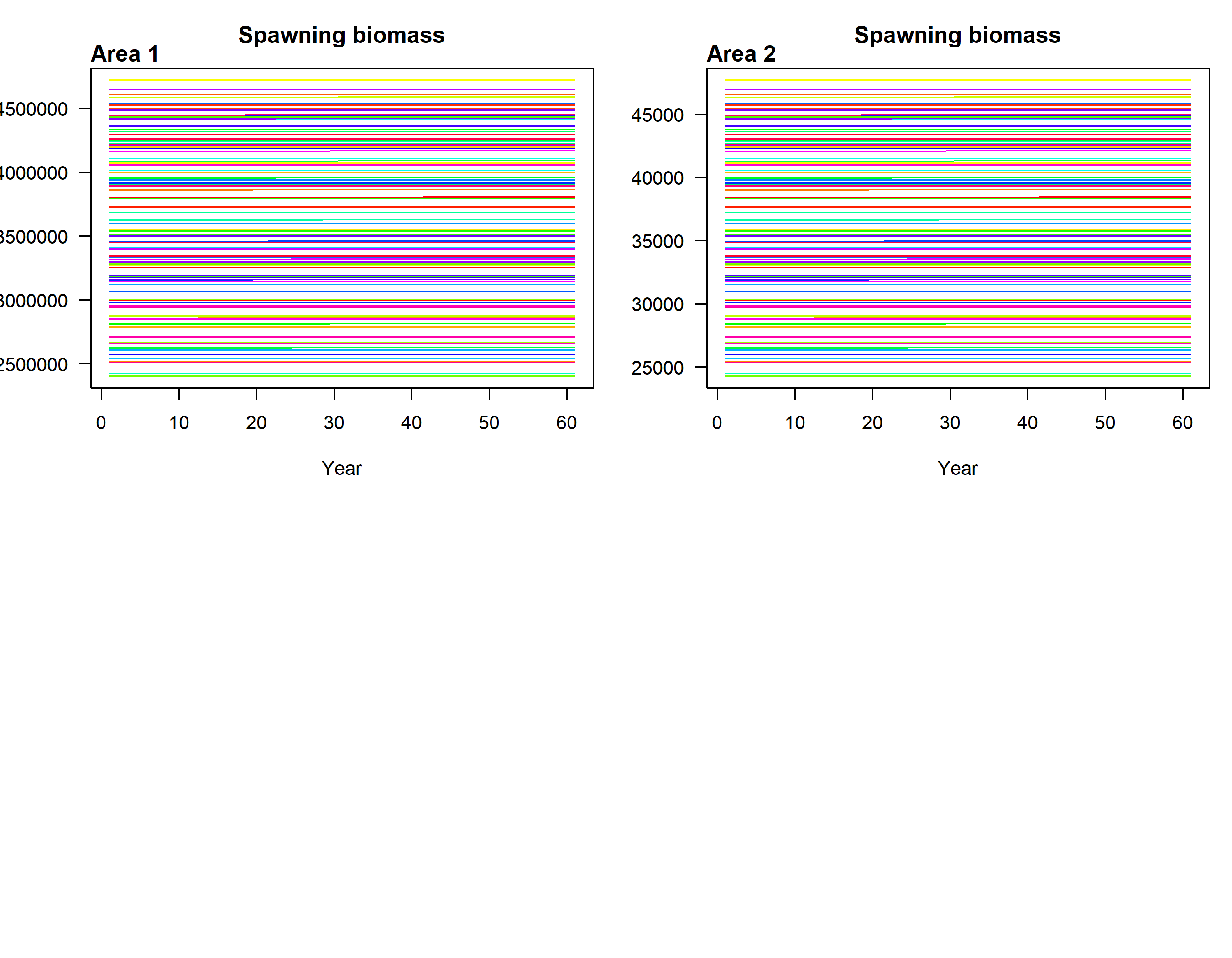
Figure 4.1: Spawning biomass by area- Higher_option1
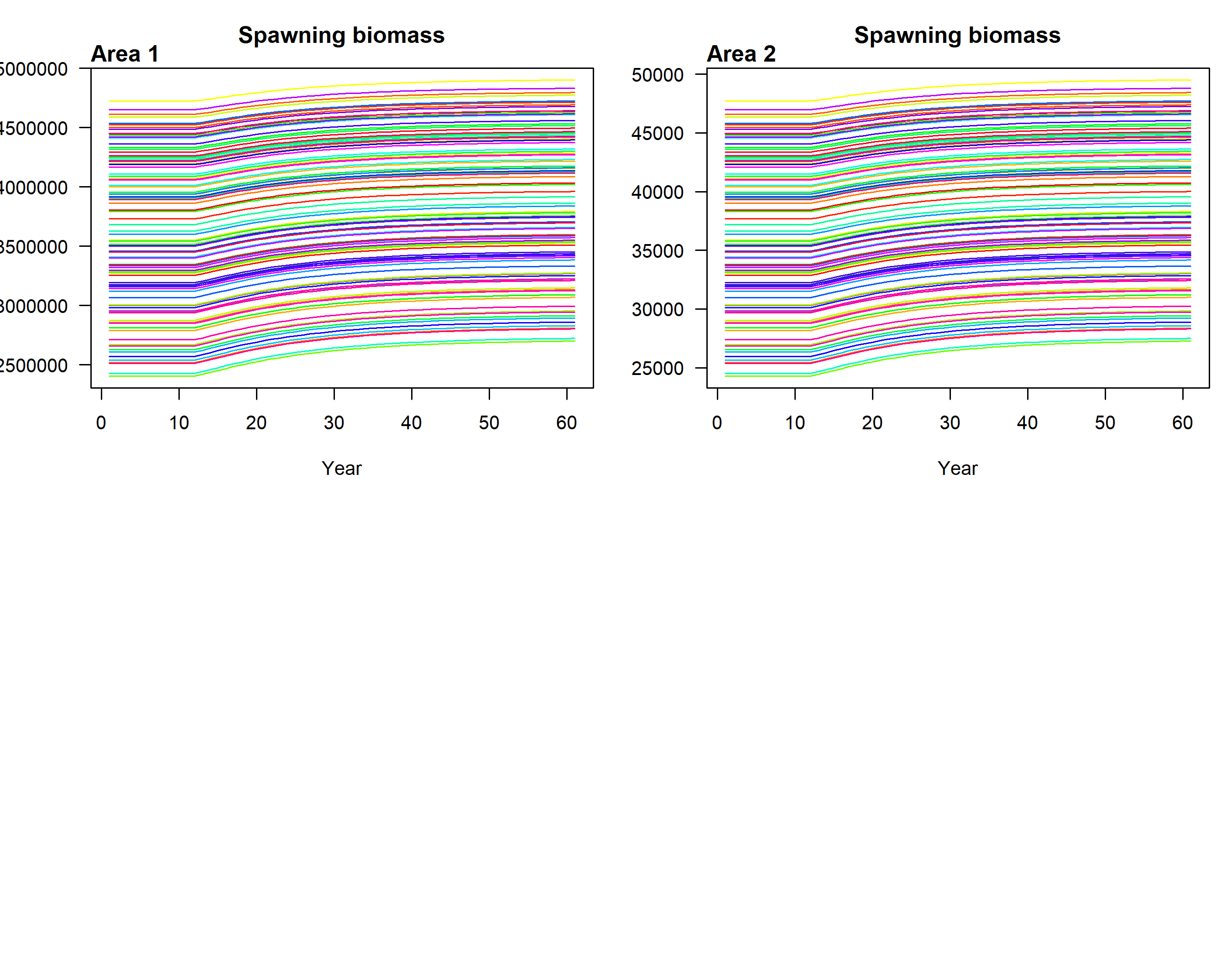
Figure 4.2: Spawning biomass by area- Higher_option2
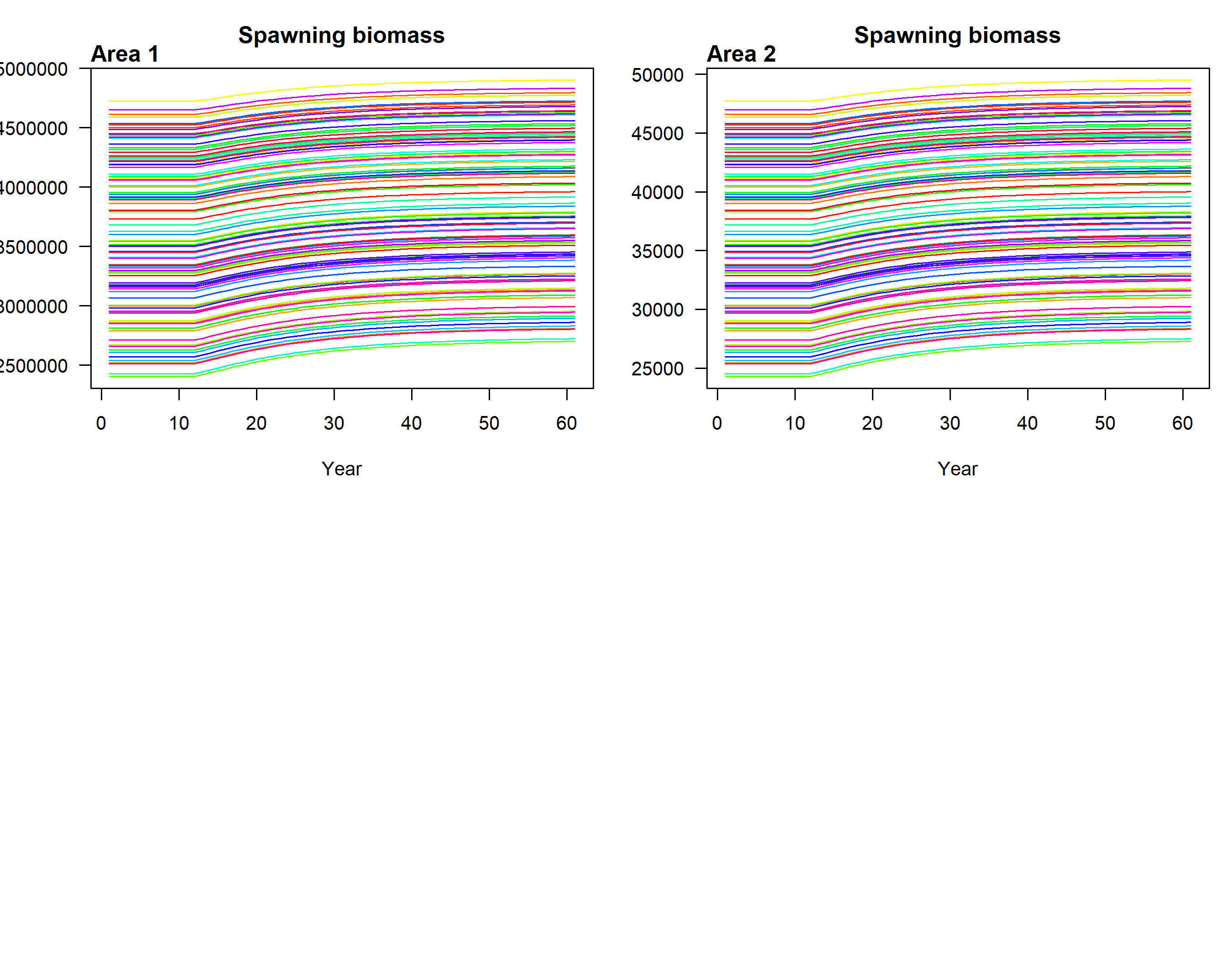
Figure 4.3: Spawning biomass by area- Higher_option3
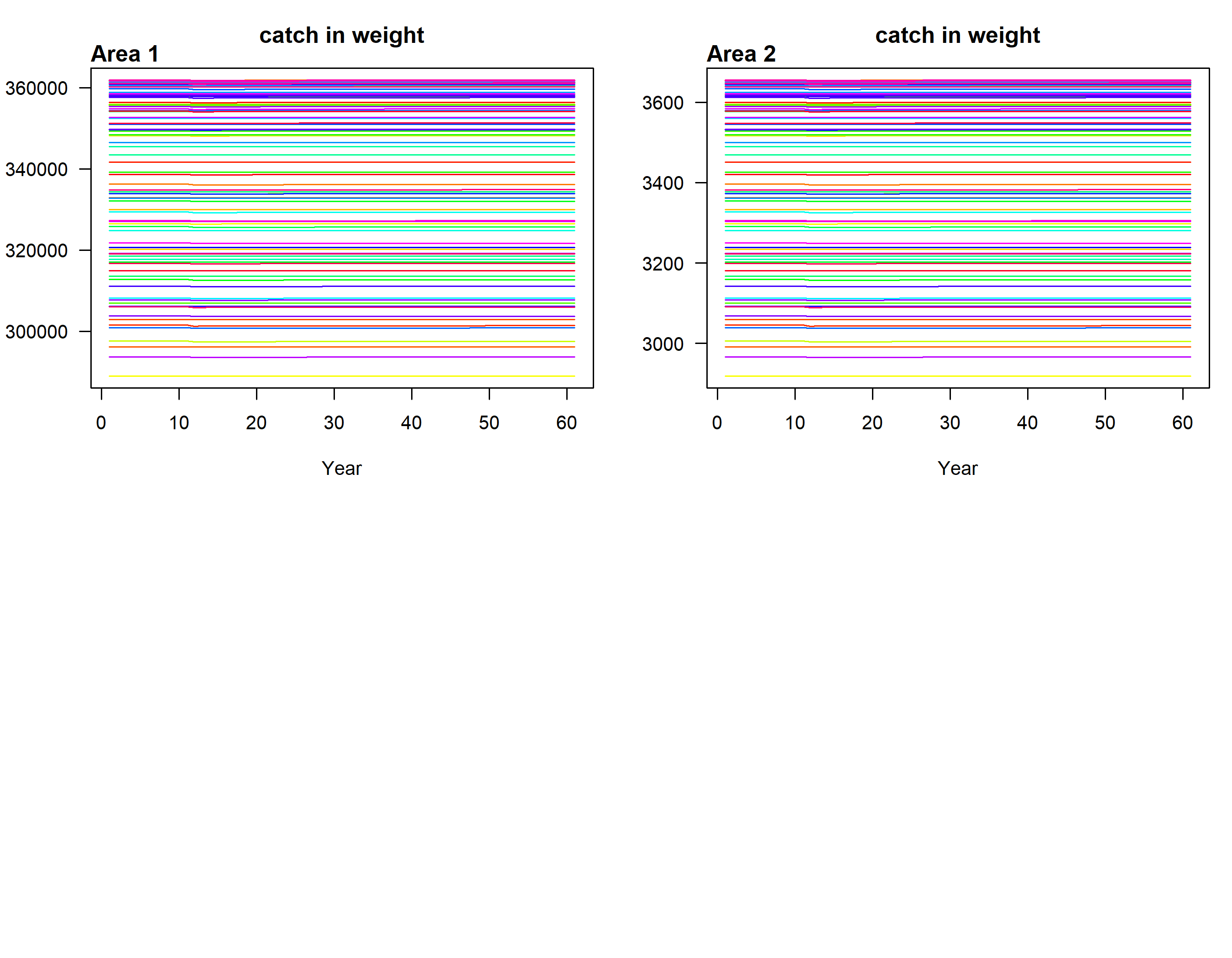
Figure 4.4: Catch biomass by area- Higher_option1
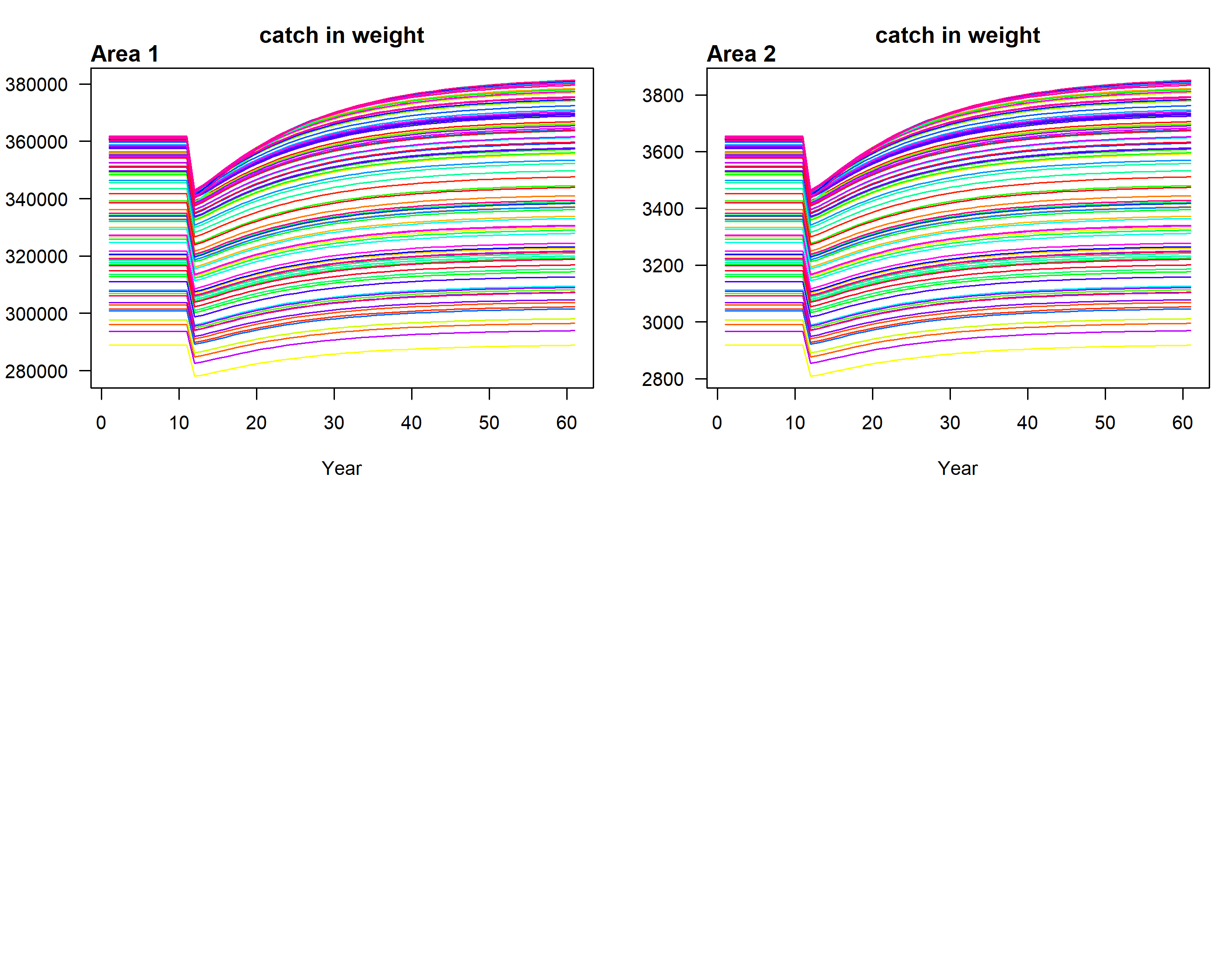
Figure 4.5: Catch biomass by area- Higher_option2
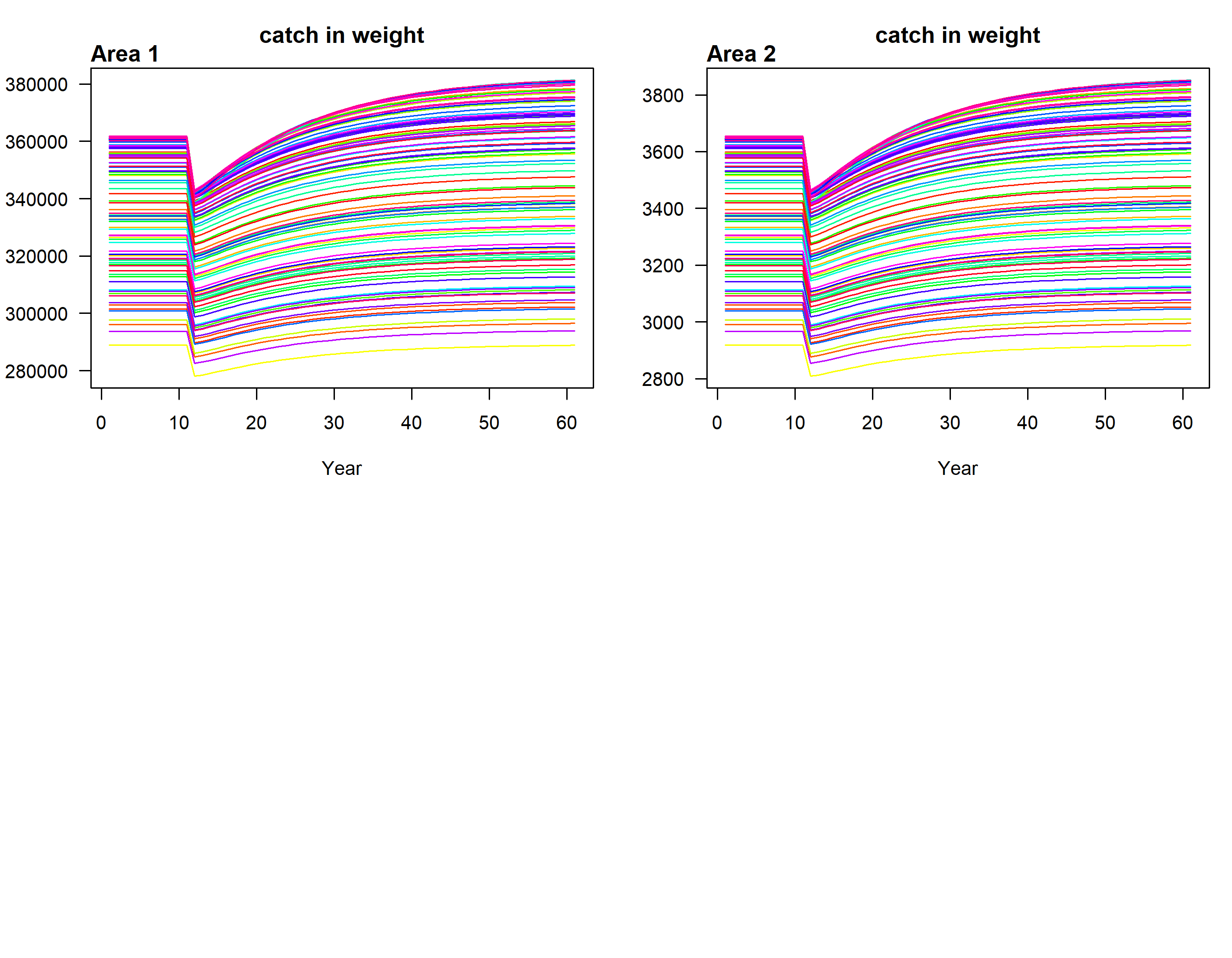
Figure 4.6: Catch biomass by area- Higher_option3